Predicting bulk moduli with matminer
Fit data mining models to ~6000 calculated bulk moduli from Materials Project
Time to complete: 30 minutes
This notebook is an example of using the MP data retrieval tool retrieve_MP.py to retrieve computed bulk moduli from
the materials project databases in the form of a pandas dataframe, using matminer’s tools to populate
the dataframe with descriptors/features from pymatgen, and then fitting regression models from the scikit-learn library to
the dataset.
Preamble
Import libraries, and set pandas display options.
# filter warnings messages from the notebook
import warnings
warnings.filterwarnings('ignore')

import numpy as np
import pandas as pd

# Set pandas view options
pd.set_option('display.width', 1000)
pd.set_option('display.max_columns', None)
pd.set_option('display.max_rows', None)
Step 1: Use matminer to obtain data from MP (automatically) in a “pandas” dataframe
Step 1a: Import matminer’s MP data retrieval tool and get calculated bulk moduli and possible descriptors.
from matminer.data_retrieval.retrieve_MP import MPDataRetrieval

api_key = None   # Set your MP API key here. If set as an environment variable 'MAPI_KEY', set it to 'None'
mpr = MPDataRetrieval(api_key)     # Create an adapter to the MP Database.

# criteria is to get all entries with elasticity (K_VRH is bulk modulus) data
criteria = {'elasticity.K_VRH': {'$ne': None}}

# properties are the materials attributes we want
# See https://github.com/materialsproject/mapidoc for available properties you can specify
properties = ['pretty_formula', 'spacegroup.symbol', 'elasticity.K_VRH', 'formation_energy_per_atom', 'band_gap',
              'e_above_hull', 'density', 'volume', 'nsites']

# get the data!
df_mp = mpr.get_dataframe(criteria=criteria, properties=properties)
print 'Number of bulk moduli extracted = {}'.format(len(df_mp))
Number of bulk moduli extracted = 6023
Step 1b: Explore the dataset.
df_mp.head()
df_mp.describe()
Step 1c. Filter out unstable entries and negative bulk moduli
df_mp = df_mp[df_mp['elasticity.K_VRH'] > 0]
df_mp = df_mp[df_mp['e_above_hull'] < 0.1]
df_mp.describe()
Step 2: Add descriptors/features
Step 2a: create volume per atom descriptor
# add volume per atom descriptor
df_mp['vpa'] = df_mp['volume']/df_mp['nsites']

# explore columns
df_mp.head()
Step 2b: add several more descriptors using MatMiner’s pymatgen descriptor getter tools
from matminer.featurizers.composition import ElementProperty
from matminer.featurizers.data import PymatgenData
from pymatgen import Composition

df_mp["composition"] = df_mp['pretty_formula'].map(lambda x: Composition(x))

dataset = PymatgenData()
descriptors = ['row', 'group', 'atomic_mass',
               'atomic_radius', 'boiling_point', 'melting_point', 'X']
stats = ["mean", "std_dev"]

ep = ElementProperty(data_source=dataset, features=descriptors, stats=stats)
df_mp = ep.featurize_dataframe(df_mp, "composition")

#Remove NaN values
df_mp = df_mp.dropna()

df_mp.head()
Step 3: Fit a Linear Regression model, get R2 and RMSE
Step 3a: Define what column is the target output, and what are the relevant descriptors
# target output column
y = df_mp['elasticity.K_VRH'].values

# possible descriptor columns
X_cols = [c for c in df_mp.columns
          if c not in ['elasticity.K_VRH', 'pretty_formula',
                       'volume', 'nsites', 'spacegroup.symbol', 'e_above_hull', 'composition']]
X = df_mp.as_matrix(X_cols)

print("Possible descriptors are: {}".format(X_cols))
Possible descriptors are: ['formation_energy_per_atom', 'band_gap', 'density', 'vpa', 'mean X', 'mean atomic_mass',
'mean atomic_radius', 'mean boiling_point', 'mean group', 'mean melting_point', 'mean row', 'std_dev X',
'std_dev atomic_mass', 'std_dev atomic_radius', 'std_dev boiling_point', 'std_dev group', 'std_dev melting_point',
'std_dev row']
Step 3b: Fit the linear regression model
from sklearn.linear_model import LinearRegression
from sklearn.metrics import mean_squared_error

lr = LinearRegression()

lr.fit(X, y)

# get fit statistics
print 'R2 = ' + str(round(lr.score(X, y), 3))
print 'RMSE = %.3f' % np.sqrt(mean_squared_error(y_true=y, y_pred=lr.predict(X)))
R2 = 0.804
RMSE = 32.558
Step 3c: Cross validate the results
from sklearn.model_selection import KFold, cross_val_score

# Use 10-fold cross validation (90% training, 10% test)
crossvalidation = KFold(n_splits=10, shuffle=True, random_state=1)

# compute cross validation scores for random forest model
scores = cross_val_score(lr, X, y, scoring='mean_squared_error',
                         cv=crossvalidation, n_jobs=1)
rmse_scores = [np.sqrt(abs(s)) for s in scores]

print 'Cross-validation results:'
print 'Folds: %i, mean RMSE: %.3f' % (len(scores), np.mean(np.abs(rmse_scores)))
Cross-validation results:
Folds: 10, mean RMSE: 33.200
Step 4: Plot the results with FigRecipes
from matminer.figrecipes.plotly.make_plots import PlotlyFig

pf = PlotlyFig(x_title='DFT (MP) bulk modulus (GPa)',
               y_title='Predicted bulk modulus (GPa)',
               plot_title='Linear regression',
               plot_mode='offline',
               margin_left=150,
               textsize=35,
               ticksize=30,
               filename="lr_regression.html")

# a line to represent a perfect model with 1:1 prediction
xy_params = {'x_col': [0, 400],
             'y_col': [0, 400],
             'color': 'black',
             'mode': 'lines',
             'legend': None,
             'text': None,
             'size': None}

pf.xy_plot(x_col=y,
           y_col=lr.predict(X),
           size=3,
           marker_outline_width=0.5,
           text=df_mp['pretty_formula'],
           add_xy_plot=[xy_params])
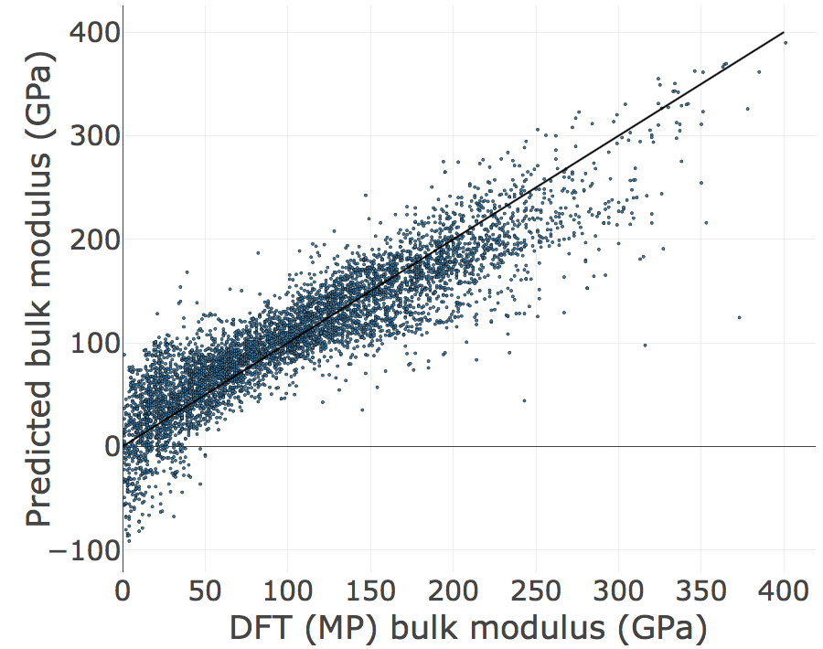
Great! We just fit a linear regression model to pymatgen features using matminer and sklearn. Now let’s use a Random Forest model to examine the importance of our features.
Step 5: Follow similar steps for a Random Forest model
Step 5a: Fit the Random Forest model, get R2 and RMSE
from sklearn.ensemble import RandomForestRegressor

rf = RandomForestRegressor(n_estimators=50, random_state=1)

rf.fit(X, y)
print 'R2 = ' + str(round(rf.score(X, y), 3))
print 'RMSE = %.3f' % np.sqrt(mean_squared_error(y_true=y, y_pred=rf.predict(X)))
R2 = 0.988
RMSE = 7.947
Step 5b: Cross-validate the results
# compute cross validation scores for random forest model
scores = cross_val_score(rf, X, y, scoring='mean_squared_error', cv=crossvalidation, n_jobs=1)

rmse_scores = [np.sqrt(abs(s)) for s in scores]
print 'Cross-validation results:'
print 'Folds: %i, mean RMSE: %.3f' % (len(scores), np.mean(np.abs(rmse_scores)))
Cross-validation results:
Folds: 10, mean RMSE: 20.087
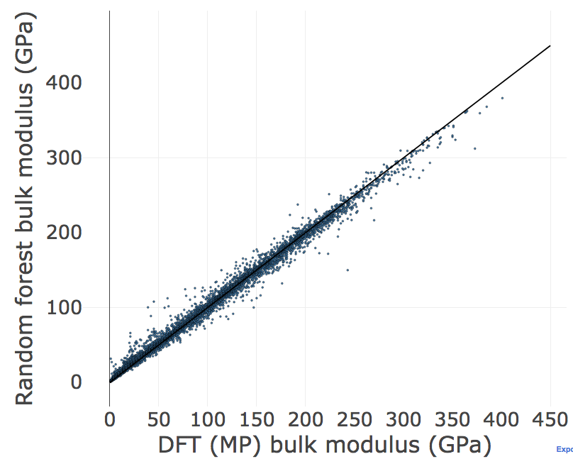
Step 6: Plot our results and determine what features are the most important
Step 6a: Plot the random forest model
from matminer.figrecipes.plotly.make_plots import PlotlyFig

pf_rf = PlotlyFig(x_title='DFT (MP) bulk modulus (GPa)',
                  y_title='Random forest bulk modulus (GPa)',
                  plot_title='Random forest regression',
                  plot_mode='offline',
                  margin_left=150,
                  textsize=35,
                  ticksize=30,
                  filename="rf_regression.html")

# a line to represent a perfect model with 1:1 prediction
xy_line = {'x_col': [0, 450],
           'y_col': [0, 450],
           'color': 'black',
           'mode': 'lines',
           'legend': None,
           'text': None,
           'size': None}


pf_rf.xy_plot(x_col=y,
              y_col=rf.predict(X),
              size=3,
              marker_outline_width=0.5,
              text=df_mp['pretty_formula'],
              add_xy_plot=[xy_line])
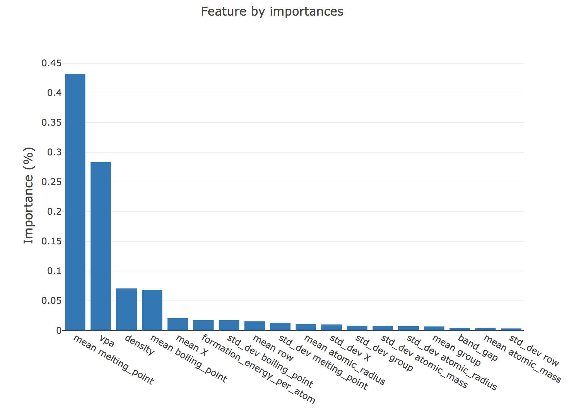
Step 6b: Plot the importance of the features we used
importances = rf.feature_importances_
X_cols = np.asarray(X_cols)
indices = np.argsort(importances)[::-1]

pf = PlotlyFig(y_title='Importance (%)',
               plot_title='Feature by importances',
               plot_mode='offline',
               margin_left=150,
               margin_bottom=200,
               textsize=20,
               ticksize=15,
               filename="rf_importances.html")

pf.bar_chart(x=X_cols[indices], y=importances[indices])